Modeling Various Air Pollutants in Cities Across the US

Project Background and Motivation

The World Health Organization reported that in 2012 about 7 million people died as a result of air pollution exposure, a finding that was more than double previous estimates. According to the WHO, this finding “confirms that air pollution is now the world’s largest single environmental health risk.” Air pollution can lead to a variety of potentially fatal conditions such as heart disease, stroke, COPD, and lung cancer. Thus it is critical that more research on air pollution causes and interventions to reduce such pollution be done.

Initial Questions:

• Are there certain pollutant profiles that characterize groups of US cities?
• What is the distribution of pollutants (air particulate matter, gas levels, etc.) within these clusters?
• What are the determinants (weather, demographics, transportation, etc.) of these pollutant profiles?
• Can we use data on weather, demographics, and transportation to predict pollutant concentrations of cities in the US?

Note: In this analysis we use the word city to refer to a core-based statistical area (CBSA) which is defined as an urban center of at least 10,000 people and the adjacent areas that are tied to the city by commuting

Key Findings

• Airborne NO₂, PM2.5, and O₃ of cities can be somewhat predicted based on demographic and weather features, but PM10, CO, and SO₂ are not well described from these characteristics.
• Prediction models based on US cities do not extend well to French cities for the pollutants that we can best predict.
• The relative importance and relationship of anthropogenic and environmental factors to air pollutants varies -- there is unlikely one key intervention to improve overall air quality.
• Distinct types of cities exist that can be characterized by their particular pollutant profiles. Cities with similar profiles may benefit from similar inteventions
• These clusters can be differentiated by liquid precipitation, air pressure, temperature, and land area.
• Imputation of cluster identities for US cities with missing data allows us to increase the coverage of the country, and seems to be fairly reliable.
• When French cities were clustered with the same method, their pollutant profiles looked reasonably similar to the clustered US pollutant profiles suggesting some generalizability beyond the US.

Analysis

Pollutant Data: The six main pollutants included in our analyis are distributed somewhat differently across the US. The interactive visualization allows you to toggle through the six pollutants to get a sense of how they are distributed. NO₂ shows clear concentrations in more urban areas which is to be expected as a primary source is car exhaust. O₃ concentrations are higher in western areas where temperatures are higher and weather is drier -- consistent with known factors contributing to ozone levels. PM2.5 may have higher concentrations in the midwest and PM10 levels are higher in the southwest. There are other patterns that can be found simply by toggling through the 6 pollutants.

Transit Data: The following plot shows the distribution of transportaion modes across different areas. The shading in the back represents the total number of people in the area. The pies have split the percentage of people who commute using each of the transportation styles listed. You can scroll over the individual pies to get the numbers, zoom in and out, or move around the area to better explore the data. In general, the most dominant form of transportation is driving alone.

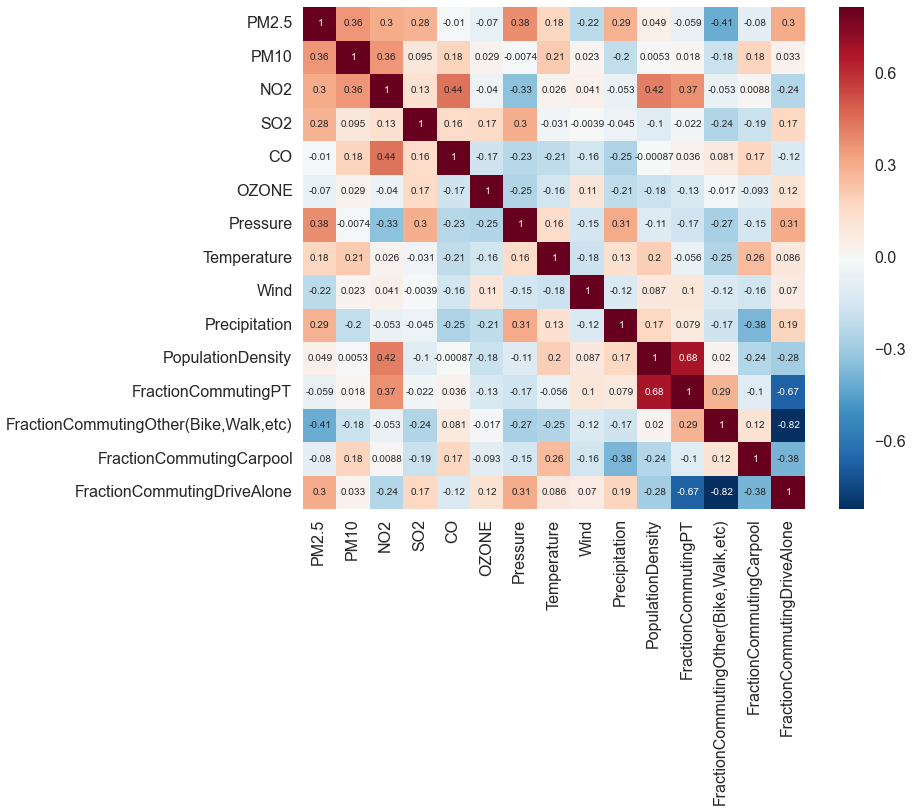
Relationships Between Pollutants and Other Factors: Given differences in pollutants across these different CBSAs, we can look to see how demographic and weather variables contribute to the observed pollutant concentrations. The following heatmap shows correlations between various predictors and pollutants. The darker the shading, the stronger the relationship -- red indicates a positive relationship and blue an inverse relationship.

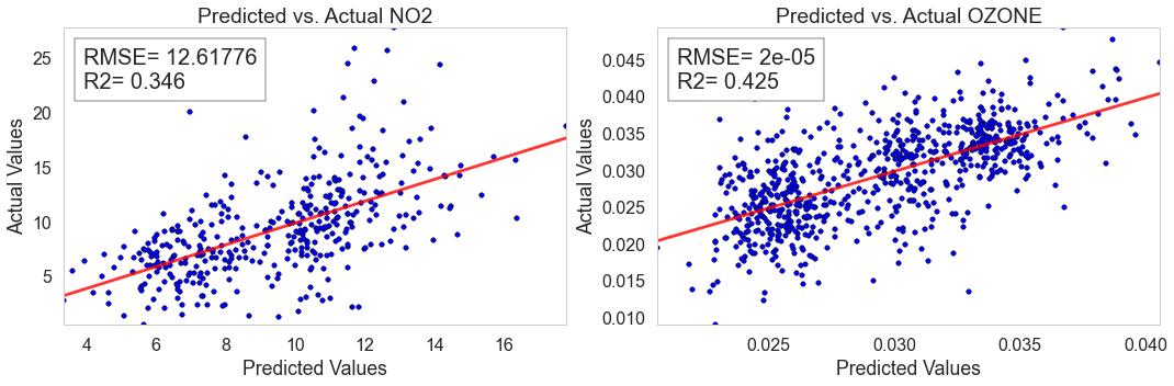
Predicting Pollutants: Models were developed to predict pollutant concentrations in cities based on demographic factors and weather. In general, the models were not completely successful, but we could predict NO₂ and ozone with relative accuracy. The predicted values for each observation are plotted against their true values in the figure below.

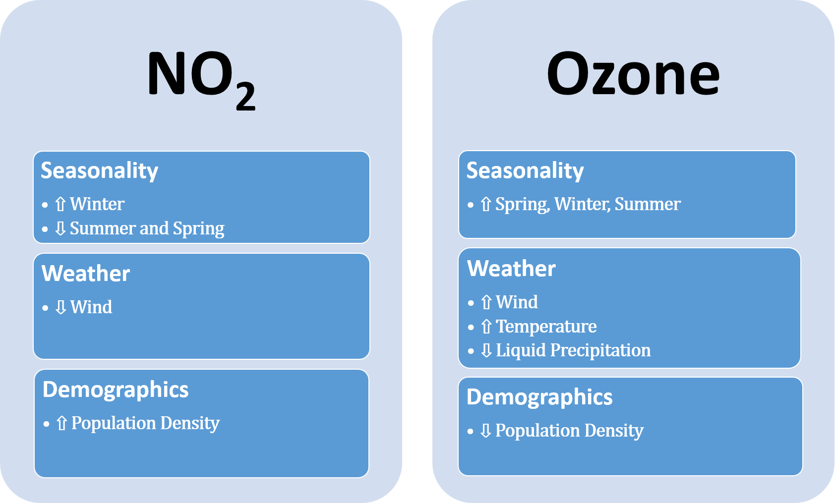
Anthropogenic vs. Natural Contributions: Understanding the relative contribution of anthropogenic and demographic factors to pollution concentrations has implications for designing appropriate regulation. To address this question, we developed multivariate models using Generalized Estimating Equations (GEE) for the most promising pollutants, NO₂ and ozone. In general, the contributions of different weather and demographic variables differ based on the particular pollutant making interventions to target overall air quality challenging.

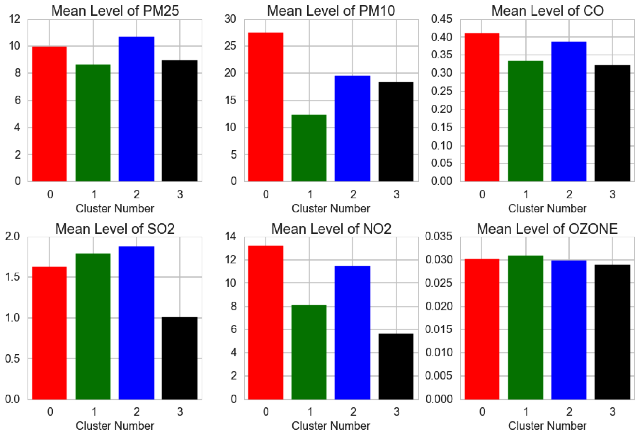
Clustering of US CBSAs: There are four distinct clusters of CBSAs in our data based on their pollutant profiles across the six key pollutants of NO₂, PM2.5, O₃, PM10, CO, and SO₂. These clusters were found using multiple iterations of k-means on the 80 CBSAs with complete pollutant data. The color-coded clusters are shown on the map below.

These clusters are statisitically significantly different in terms of pollutant profiles with PM10 and NO2 levels most significantly differentiating the clusters. The below graph allows you to see how the clusters differ in terms of the mean level of the pollutants.

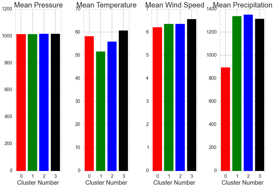
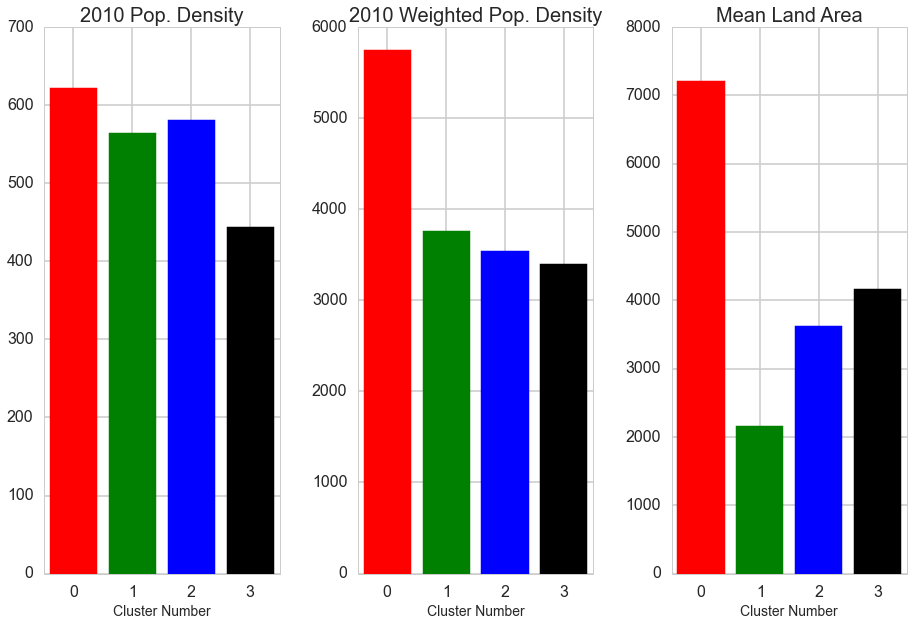
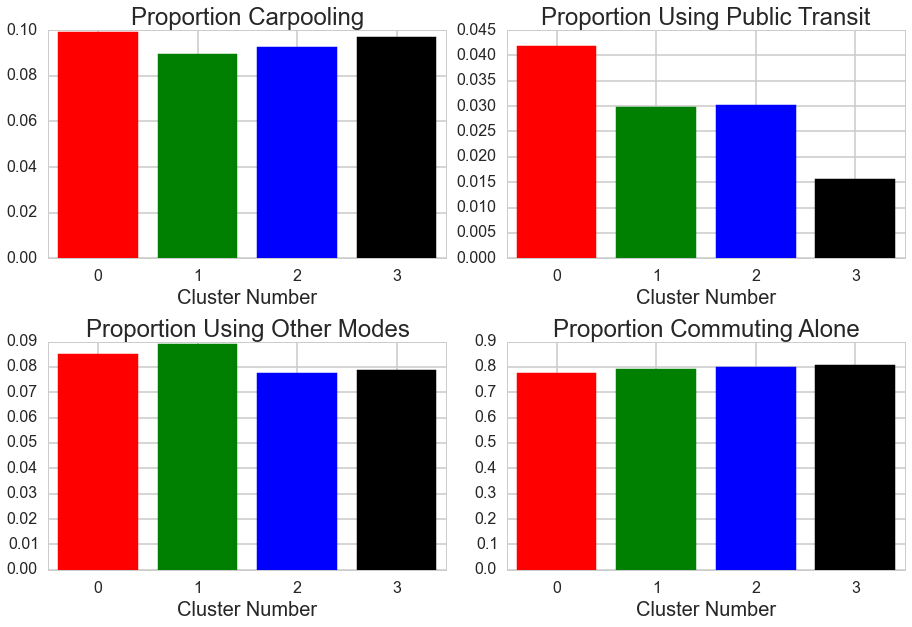
It was of interest to determine if these four clusters differ significantly in predictors of air pollution such as weather patterns, commuting patterns, and/or population variables. Statistical testing showed that these clusters differ in their profiles of determinants with land area, average air pressure, average yearly temperature, and average yearly precipitation significantly differentiating the clustering. You can see the differences in these determinants among clusters in the below graphs.

Expanding Clusters to More US CBSAs: As we were only able to cluster the 80 CBSAs with complete pollutant data in generating the profiles above, we applied K-Nearest Neighbors to impute the cluster label of cities that were missing data for 1 or 2 pollutants. In theory, the CBSA should get the label that most of the cities with similar concentrations of pollutants. When this was done, we were able to increase our number of CBSAs in a cluster from 80 to 186. The visual below shows the increase.

When looking at the pollutant profiles of the imputed clusters, we see that it is fairly similar to the profiles in the original clusters, indicating that our method of imputation using k-nearest neighbors was likely to be successful.

However, when looking at the other determinants (for weather, population, and transportation), the profiles changed compared to the original clusters (see github for more details). This change may have occurred because of the rather large number of cities that were added to the analysis. By imputation, we more than doubled the number of cities included.

Finally, we tried to extend our clusters made from the US data to foreign data, namely from France. This was done by using the same method as before (k-nearest neighbors imputation). All of the French cities that we clustered only fell into two clusters (Cluster 0 and 2). The clustering of the French cities is difficult to examine because of the only 2 clusters represented -- it could be that French cities only fall into two types of US clusters, or we just don't have enough variation in French cities in the current dataset. We would want to add additional cities to our analysis, preferably from across Europe to increase variation in the data and obtain more diverse cluster assignments.

Future Directions

The analysis presented here is not without limitations. Our best predictive model could only explain about 45% of the variation in ozone leaving much unexplained. Furthermore, in validating these predictive models we saw that in general models built on US data did not perform well in France. Beyond the predictive modeling, issues with missing data for pollutants made clustering cities into distinct pollutant profiles challenging. In the future, steps what would be helpful would be to:

1. Collect more predictors -- this includes more weather data, data on land use (agricultural, industrial, commerical, forested, etc.), government air quality regulations, and better transportation information for the validation dataset,
2. Expand beyond the year 2010 to see if there are historical trends in air quality
3. Incorporate city-specific data rather than using CBSA units via a hierarchical model to account for localized variation in pollutant levels
4. Expand our validation set to other countries to address our current problems of small sample size and low variability and to increase generalizability of the models
5. Improve imputation of cities with missing pollutant data to increase coverage of clusters across the US
6. By including more data across years, determinants, and countries we would hope to have a robust model that could be used to inform city-specific air pollution policies

Data

All raw data can be found at the following dropbox link

In order to assess the various factors that may influence air quality in urban areas across the United States, four main data sources were required:

1. Air Quality Data
2. Historical Weather Data
3. Demographic Data
4. Transit Data

Air Quality Data:

Air Quality Data for the various Core-Based Statistical Areas (CBSA's) across the United States were obtained from the EPA's AirData repository. Data was downloaded for the six key pollutants for the year of 2010.

Historical Weather Data:

US weather data was also obtained from the EPA's AirData repository. This includes information of daily temperature, wind speeds, relative humidity, and atmospheric pressure. A secondary source of weather data came from the National Oceanic and Atmospheric Administration (NOAA). Using their FTP site, more detailed breakdown of weather data including wind speeds, temperature, atmospheric pressure, and daily precipitation could be obtained for various stations across the US. This helped fill in missing data and get a finer image of US weather.

Demographic Data:

Demographic information for the CBSA's included in this research came from the US Census Bureau. These files contain information about the total population, the total land area, and the population density of CBSAs in the year 2010.

Transit Data:

To assess the influence of commuting style on pollutant levels, data on mode of commuting were collected from the 2010 US Census Bureau. These data included breakdown of commuters' modes of transportation into 'Driving Alone,' 'Carpooling,' 'Public Transportation,' and 'Other (Walk/Bike/etc.).'

Github Repository

The analysis for this project can be found at the following github repository. The optimal way to navigate the various ipython notebooks is as follows

1. Prologue.ipynb
2. DataCollection&Cleaning.ipynb
3. ExplotatoryDataAnalysis.ipynb
4. PredictiveLinearModeling.ipynb
5. UnsupervisedAnalysis.ipynb
6. UnsupervisedLearning_pt2.ipynb